Analysis

This section describes the technical evolution of the navigation and estimation subsystems, including the original state-space observer approach with IMU fusion, the issues encountered during implementation, and the final displacement-based odometry solution that enabled reliable autonomous navigation.

Original Approach: State-Space Observer with IMU Fusion

System Model and Kinematics

The original navigation system implemented a continuous kinematic state estimator combining encoder-derived wheel velocities with IMU-derived absolute heading. The approach was grounded in differential drive kinematics and numerical integration using a 4th-order Runge-Kutta (RK4) solver.

State Vector and Dynamics

The observer estimated a 6-state vector representing the robot’s configuration and motion:

\[\begin{split}\mathbf{x} = \begin{bmatrix} X \\ Y \\ \theta \\ s \\ \Omega_L \\ \Omega_R \end{bmatrix}\end{split}\]

where:

• \(X, Y\) = global position in the plane (meters)

• \(\theta\) = robot orientation (radians)

• \(s\) = arc length traveled (meters)

• \(\Omega_L, \Omega_R\) = left and right wheel angular velocities (rad/s)

The state dynamics were derived from the differential drive kinematic model:

\[\begin{split}\dot{X} &= \frac{r}{2}(\Omega_R + \Omega_L)\cos(\theta) \\ \dot{Y} &= -\frac{r}{2}(\Omega_R + \Omega_L)\sin(\theta) \\ \dot{\theta} &= \frac{r}{w}(\Omega_R - \Omega_L) \\ \dot{s} &= \frac{r}{2}(\Omega_R + \Omega_L)\end{split}\]

The motor velocity dynamics were modeled as first-order systems driven by applied voltages:

\[\begin{split}\dot{\Omega}_L &= \frac{1}{\tau}\left(\frac{K}{N}u_L - \Omega_L\right) \\ \dot{\Omega}_R &= \frac{1}{\tau}\left(\frac{K}{N}u_R - \Omega_R\right)\end{split}\]

where \(K\) is the motor gain constant, \(\tau\) is the motor time constant, \(N\) is the gear ratio, and \(u_L, u_R\) are the commanded motor voltages.

IMU Integration and Heading Correction

Rather than relying solely on integrated encoder differential to estimate heading, the system used the BNO055 IMU to provide absolute orientation. The IMU heading was low-pass filtered and corrected for initial offset:

\[\theta_\mathrm{corrected} = \alpha \cdot \theta_\mathrm{IMU} + (1-\alpha) \cdot \theta_\mathrm{prev}\]

where \(\alpha = 0.3\) was the filter coefficient. This fusion approach reduced heading drift that would otherwise accumulate from encoder noise and wheel slip.

Velocity Estimation from Encoders

Encoder ticks were converted to linear wheel velocities using:

\[v = \frac{\Delta \mathrm{ticks}}{\Delta t} \cdot \frac{C_\mathrm{wheel}}{N_\mathrm{ticks}} \cdot 10^6 \cdot k_\mathrm{scale}\]

where \(C_\mathrm{wheel}\) is the wheel circumference, \(N_\mathrm{ticks}\) is encoder resolution, \(\Delta t\) is in microseconds, and \(k_\mathrm{scale}\) is an empirical velocity correction factor.

RK4 Numerical Integration

The state estimate was propagated forward in time using a 4th-order Runge-Kutta integrator with 10 substeps of 10 ms each, for a total horizon of 100 ms per observer cycle. The RK4 algorithm is:

\[\mathbf{x}_{n+1} = \mathbf{x}_n + \frac{1}{6}\left(\mathbf{k}_1 + 2\mathbf{k}_2 + 2\mathbf{k}_3 + \mathbf{k}_4\right) \Delta t\]

where:

\[\begin{split}\mathbf{k}_1 &= \mathbf{f}(t, \mathbf{x}_n) \\ \mathbf{k}_2 &= \mathbf{f}\left(t + \frac{\Delta t}{2}, \mathbf{x}_n + \frac{\mathbf{k}_1 \Delta t}{2}\right) \\ \mathbf{k}_3 &= \mathbf{f}\left(t + \frac{\Delta t}{2}, \mathbf{x}_n + \frac{\mathbf{k}_2 \Delta t}{2}\right) \\ \mathbf{k}_4 &= \mathbf{f}(t + \Delta t, \mathbf{x}_n + \mathbf{k}_3 \Delta t)\end{split}\]

This approach provided substantially better accuracy than Euler integration for the same step size.

IMU Subsystem Architecture

BNO055 Driver and Communication

The IMU subsystem used a custom bit-banged I²C implementation (SoftI2C) to communicate with the BNO055 sensor. This design choice was made to:

• Provide explicit control over bus timing and recovery

• Implement retry logic for transient communication failures

• Support bus recovery if SDA or SCL became stuck

The driver implemented START/STOP condition generation, ACK/NACK handling, and register read/write primitives with automatic retry and recovery.

Calibration Persistence

The BNO055 requires calibration of its magnetometer, accelerometer, and gyroscope. To avoid recalibrating on every boot, the system stored the 22-byte calibration blob to a text file (calibration.txt) encoded as a hex string. On startup:

1. The calibration file was checked for existence

2. If found, the blob was decoded and written to the IMU registers

3. If not found, the user performed manual calibration by rotating the robot until the sensor reported full calibration (sys = 3)

4. The new calibration blob was saved for future boots

This ensured consistent sensor performance across power cycles.

IMU Handler Task and Startup FSM

The IMU handler task represents inertial sensor management over I2C, including initialization, calibration management, and data readiness. It is responsible for bringing the IMU into a known operating mode and ensuring that usable heading or yaw rate information is available to other tasks. Calibration persistence is handled by loading a saved calibration blob when present, and saving new calibration data after a successful manual procedure so repeated runs can start quickly with consistent sensor behavior.

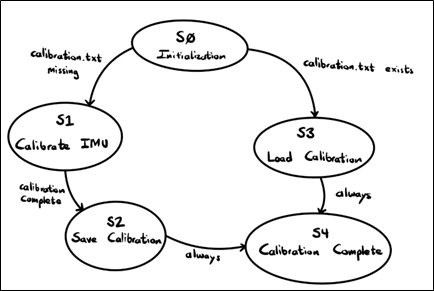
IMU handler FSM performing BNO055 reset, calibration load or manual calibration, calibration persistence, and steady state data readiness over I2C.

A dedicated startup task managed the full IMU initialization and calibration sequence as a finite state machine:

1. Hardware Reset: Toggle the IMU reset pin

2. I²C Initialization: Establish communication

3. Calibration File Check: Load stored calibration if available

4. Manual Calibration: Enter calibration mode if needed

5. Calibration Save: Persist new calibration data

6. Ready State: Enable navigation and observer tasks

During initialization the task performs a reset sequence and brings up the I2C interface. It then checks for stored calibration data and loads it to avoid repeated manual calibration. If no valid calibration exists, it enters a manual calibration mode that monitors calibration status until completion, then saves the calibration blob for future boots. Once complete, the task remains in a steady state where inertial measurements can be sampled consistently and provided to the rest of the system through shared variables.

This encapsulated all IMU readiness concerns into a single subsystem, preventing downstream tasks from running until the sensor was fully operational.

IMU Monitor Task

After calibration, a periodic task extracted:

• Continuous heading (unwrapped across 0–360° boundaries)

• Yaw rate (angular velocity)

These values were published to shared variables consumed by the controller and navigation tasks.

Observer Task

The observer task represents model based state estimation implemented in state space form. It runs concurrently with the control stack, using measured outputs and applied inputs to estimate internal states that are not directly measured or that benefit from filtering. The observer gain is selected using pole placement to achieve stable convergence behavior, and RK4 integration is used to propagate the state estimate forward in time under the discrete task period.

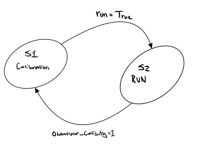
Observer structure showing state space estimation with Luenberger gain injection and RK4 integration under a discrete task period.

This task formalizes estimation as part of the architecture rather than ad hoc filtering. By publishing estimated states through shares, the observer output can be consumed by other tasks without changing their hardware interfaces, allowing estimation improvements to be integrated cleanly into navigation or control when required by the course segment or sensing constraints.

Navigation with State Estimation

The original navigation logic used the observer’s \(X, Y\) position estimates and IMU heading to make state-based decisions. A typical navigation sequence included:

State 0 — Biased Line Following

• Enable line following with a leftward bias once \(X > 550\) mm

• Used for fork or branch selection

State 1 — Heading Adjustment

• Trigger when \(Y\) exceeded a threshold

• Command a target heading (e.g., 90°)

• Set nav_turn_flg = 1 to enable heading-based control

State 2 — Straight IMU-Controlled Motion

• Disable line following

• Maintain forward motion using IMU heading (force-straight mode)

State 3 — Resume Line Following

• Re-enable line tracking with zero bias after reaching another \(Y\) threshold

This approach combined sensor fusion with line following to handle multi-segment courses requiring precise positioning and orientation control.

Reference Implementation

The complete original implementation is preserved with the defunct_ prefix in src/ and includes:

• defunct_observer_fcn.py — State-space dynamics and output equations

• defunct_rk4_solver.py — 4th-order Runge-Kutta integrator

• defunct_IMU_driver.py — Bit-banged I²C and BNO055 interface

• defunct_CalibrationManager.py — Calibration blob persistence

• defunct_IMU_handler.py — Startup FSM and initialization

• defunct_navigation.py — Position-based navigation logic

• defunct_main.py — Task coordination and scheduler setup

See also

Full API documentation for these modules is available in Original Approach API Reference.

Issues Encountered and Pivot to Displacement-Based Approach

IMU Communication Reliability

The team invested substantial effort into making the IMU-based approach work reliably. This included implementing sophisticated retry logic, bus recovery mechanisms, and extensive calibration management infrastructure. Despite these efforts and many hours of debugging and refinement, the BNO055 exhibited intermittent I²C communication failures during critical phases of the run. These failures manifested as:

• Register read timeouts mid-trial

• Incorrect heading values due to incomplete transactions

• Bus lockup requiring hardware reset

Through systematic debugging with oscilloscope measurements and logging, the root cause was traced to timing sensitivity in the bit-banged I²C implementation combined with electromagnetic interference from motor PWM and power supply transients. While the system worked reliably in static conditions and benchtop testing, dynamic motor operation introduced sufficient noise to corrupt I²C transactions unpredictably. Multiple attempts were made to resolve this through improved shielding, I²C timing adjustments, and filtering, but the reliability issues persisted under full operational conditions.

Calibration Drift and Magnetic Interference

Even when communication was stable, the magnetometer-based heading output drifted over time due to:

• Nearby ferromagnetic materials in the course environment

• Motor current-induced magnetic fields

• Difficulty achieving sys = 3 calibration consistently in the competition setting

This drift caused the position estimate to accumulate error over the course of a trial, particularly during segments requiring precise turns or distance-based transitions.

Decision to Refactor

After extensive troubleshooting and multiple attempts to achieve reliable IMU operation, the team made the difficult decision to pivot to a simpler displacement-based odometry approach. This was not an abandonment of the sophisticated state estimation framework, but rather a pragmatic response to persistent hardware reliability issues that could not be resolved within project time constraints. The substantial groundwork in observer design, sensor fusion theory, and RK4 integration provided valuable insights that informed the final implementation. The decision prioritized:

• Reliability over theoretical optimality

• Encoder-only state estimation with known accuracy

• Removal of I²C communication as a single point of failure

• Preservation of lessons learned from the observer-based approach

Final Approach: Displacement-Based Odometry

Encoder Heading and Distance Estimation

The final system implemented a pure encoder-based odometry estimator using differential drive kinematics. The encoder heading task runs as a continuous periodic loop, computing heading and distance from left and right wheel motion.

Distance Calculation

Forward distance traveled is computed as the average displacement of both wheels:

\[d = \frac{d_L + d_R}{2}\]

where each wheel displacement is:

\[d_i = \frac{\Delta \mathrm{ticks}_i}{N_\mathrm{ticks}} \cdot C_\mathrm{wheel}\]

Heading Calculation

Heading change is computed from the differential wheel displacement:

\[\Delta \theta = \frac{d_R - d_L}{w}\]

where \(w\) is the track width. The heading is integrated over time and normalized to \([-180°, 180°]\) using unwrapping logic to handle discontinuities at \(\pm 180°\).

Unwrapping and Normalization

To prevent heading discontinuities from causing control errors, the algorithm applies unwrapping:

\[\delta = \theta_\mathrm{new} - \theta_\mathrm{prev}\]

If \(\delta > 180°\), subtract \(360°\). If \(\delta < -180°\), add \(360°\). The continuous heading is then accumulated and re-normalized into the bounded range.

Navigation Using Displacement Thresholds

The navigation FSM transitioned from position-based (\(X, Y\)) logic to distance-based thresholds. Each state transition is triggered when the cumulative distance exceeds a calibrated value, combined with heading error checks to ensure orientation accuracy before proceeding.

This approach proved significantly more reliable because:

• Encoder distance is monotonically increasing and does not drift

• Heading error can be bounded by resetting odometry at known course features

• No external sensor dependencies introduce failure modes

Comparison to Original Approach

Aspect	Original (State-Space + IMU)	Final (Displacement-Based)
State Estimation	6-state RK4 observer	Direct encoder integration
Heading Source	BNO055 IMU (absolute)	Encoder differential (relative)
Position Estimate	Global \(X, Y\) (meters)	Cumulative distance (mm)
Sensor Fusion	IMU + encoders	Encoders only
Communication Dependency	I²C (bit-banged)	None (encoders via hardware timer)
Drift Characteristics	Magnetometer drift over time	Heading drift from wheel slip
Reliability	Intermittent I²C failures	Highly reliable
Complexity	High (RK4, IMU driver, calibration)	Low (kinematic equations only)

The displacement-based approach sacrificed global position awareness in favor of robustness and repeatability, which proved to be the correct tradeoff for the obstacle course navigation task.

Bluetooth Telemetry and Line Following Breakthrough

A key capability that accelerated our progress was real time introspection of the running firmware. After integrating the Bluetooth module, we streamed structured REPL output to a PC using PuTTY while Romi executed its cooperative tasks. This gave us continuous visibility into internal variables such as encoder velocity, PI error, integrator state, line centroid, saturation status, and scheduler state flags. With that visibility, each trial became a measurable experiment. We could confirm timing behavior, detect mode transitions, validate that calibration was applied correctly, and save full text logs for offline plotting and direct comparison across runs.

From there, we focused on the most control intensive milestone of the term: stable line following with the 7 channel Pololu QTR array. The program treats line tracking as a closed loop regulation problem driven by a centroid measurement computed from the reflectance profile. Each sample produces a normalized set of sensor intensities, a centroid location across the array, and a signed lateral error relative to the center sensor. That error is then converted into a steering correction which is injected into the motor effort commands while the underlying velocity loop maintains repeatable forward speed.

Control and sensing were implemented explicitly in the code using the following sequence of computations.

IR calibration and normalization

Calibration establishes two reference measurements for each channel, one for white background and one for black tape. During runtime, each raw reading is mapped into a normalized intensity so the centroid calculation remains consistent across lighting variation and across repeated trials.

\[I_i = \mathrm{clip}\!\left(\frac{R_i - W_i}{B_i - W_i},\,0,\,1\right)\]

where \(R_i\) is the raw sensor reading for channel \(i\), \(W_i\) is the white reference, \(B_i\) is the black reference, and \(I_i\) is the normalized intensity used for line tracking.

Centroid and line error

The centroid represents the weighted location of the detected line across the array. With seven sensors indexed left to right, the centroid is computed as:

\[c = \frac{\sum_{i=1}^{7} p_i I_i}{\sum_{i=1}^{7} I_i}\]

where \(p_i\) are the sensor position weights. The signed line error is then formed relative to the desired center position \(c_0\):

\[e_\mathrm{line} = c - c_0\]

This single scalar error gives the controller a continuous measure of how far the line is from the center of the array, with sign indicating which direction the robot must steer to recenter.

Velocity PI control and steering injection

Each wheel is regulated using a PI velocity controller driven by encoder speed feedback. The core loop follows:

\[e_v(t) = v_\mathrm{ref}(t) - v(t)\]

\[u_\mathrm{PI}(t) = K_p e_v(t) + K_i \int e_v(t)\,dt\]

The line following correction is implemented as an additive differential term that biases left and right effort in opposite directions:

\[\Delta u_\mathrm{line}(t) = K_\ell e_\mathrm{line}(t) + K_{\ell i}\int e_\mathrm{line}(t)\,dt\]

\[u_L(t) = \mathrm{sat}\!\left(u_\mathrm{PI}(t) - \Delta u_\mathrm{line}(t)\right), \quad u_R(t) = \mathrm{sat}\!\left(u_\mathrm{PI}(t) + \Delta u_\mathrm{line}(t)\right)\]

where \(u_L\) and \(u_R\) are the left and right motor effort commands and \(\mathrm{sat}(\cdot)\) enforces the allowable effort range. This structure makes the behavior interpretable during tuning because the forward speed is controlled by the velocity loop while lateral correction is controlled by the centroid error terms.

Integrator management and repeatability

To maintain stability across aggressive maneuvers, the program tracks saturation and constrains integral accumulation when the output is pinned at its limit. This prevents integrator growth from dominating the response after the robot reacquires the line. The same philosophy is applied to the line integral term so that line correction remains smooth rather than accumulating a large bias during temporary loss of contrast.

Tuning workflow and physical validation

At this phase of the term, most iteration time was spent converting these computations into reliable physical performance. We tuned \(K_p\) and \(K_i\) for stable speed tracking, then tuned \(K_\ell\) and \(K_{\ell i}\) so the robot continuously recentered on the tape without oscillation, overshoot, or drift. Each trial around the black circle was evaluated using the telemetry stream and direct observation. We looked for the same signatures in the data every run: bounded line error, stable encoder speed, limited saturation time, and consistent centroid convergence after disturbances. Once the robot could follow the circle repeatedly, we had a validated sensing and control foundation that supported the later navigation logic used on the obstacle course.

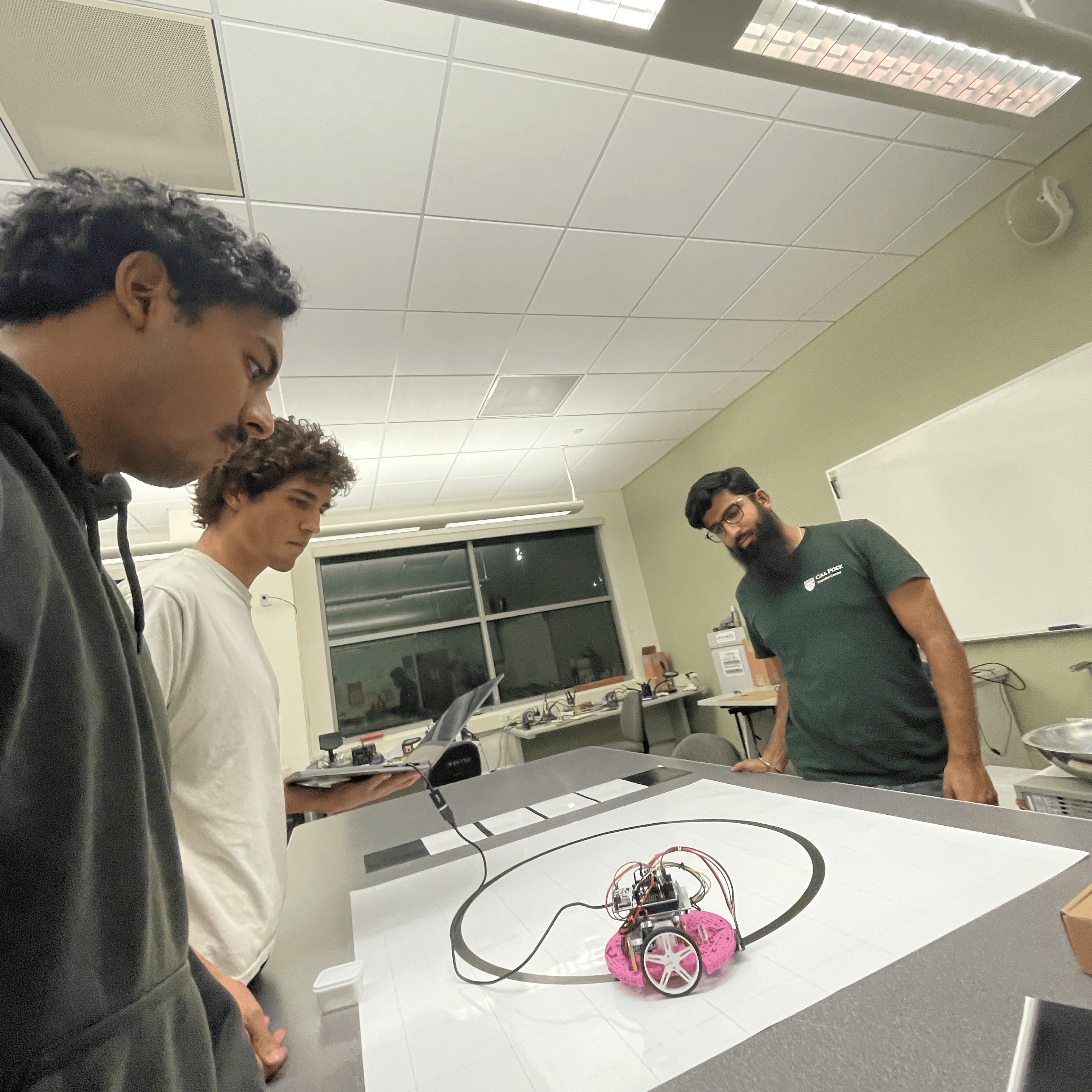
Our team during the line following tuning phase, using live PuTTY telemetry and repeated trials to refine calibration, gains, and stability margins.

First stable line following breakthrough demonstrating centroid based tracking with PI velocity regulation and continuous steering correction.